Generative Learning Algorithms
Andrew NG. So much likely I would be overwhelmed.
Imagine giving different features of two animals to logistic regression, what would we find? It determines the boundary which separates two animals and for any new instance it would compare which boundary it falls into to classify it. Let’s take this whole thing into next level.
Let’s take an example of classifying elephant and dog. What if we build a model of what elephants look like and then similar model about dogs. Finally to classify new animal, we match it against both of these models and check which one is more likely to resemble any of them.
The first approach of finding boundary values is called DISCRIMINATIVE approach. These models learn P(y|x). The second approach learns P(x|y). i.e. we are building x. Such algorithm is called GENERATIVE. If y = 0 is dog and y =1 is elephant ,then p(x|y = 1) models the distribution of elephants’ features (x).
If we are using P(y|x) to classify , we know that argmax of P(y|x) = argmax P(x|y)*P(y).
Gaussian Discriminant Analysis:
We will also look into Naive Bayes. But GDA first. This model assumes that p(X|y) has multivariate Gaussian Distribution. First we will look into multivariate Gaussian Distribution.
1.1 The multivariate normal distribution
Single Variable has mean and variance, multivariate has µ ∈ R^n and a covariance matrix Σ ∈ R^(n×n).
The probability distribution is given by:

We know that expectation is E[X] = integration(x.P(X)) in single variable normal distribution. Here it stays same.

Remember our bell shape curve of single variable normal distribution?
Here is our multivariate distribution of mean 0 and variance shown below

GDA model
We know that y is either 0 or 1 in terms of our elephants and dogs classification. So it follows Bernoulli distribution.
We have P(x|y=0) dogs distribution and P(x|y=1) elephants distribution but they follow Gaussian distribution.
So, we can write that as,

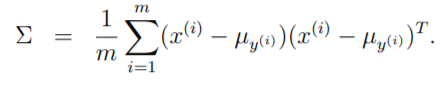
Here, the parameters of our model are φ, Σ, µ0 and µ1. Take a note that we have used same covariance matrix(Σ) for both of them.
The log likelihood is given by,

The parameters for P(X|y) are Σ, µ0 and µ1 and P(y) is φ. φ is parameter of Bernoulli distribution which is given by,


Suppose X consists of height and weight. 2 dimensional vectors. so µ0 is 2 dimensional vector of [meanOfHeight, meanOfWeight]. MeanOfHeight and MeanOfWeight for those values that give y=0 is called µ0.

GDA and Logistic Regression:
P(y=1|x) can be expressed in terms of logistic regression.
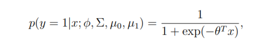
Isn’t θ a parameter just like mean, covariance and others we have seen? Yes. It is. It is the approximate function of all those parameters.
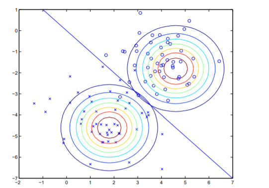
When would we prefer one model over another? GDA and logistic regression will, in general, give different decision boundaries when trained on the same dataset. Which is better?
We just argued that if p(x|y) is multivariate gaussian (with shared Σ), then p(y|x) necessarily follows a logistic function. Bernoulli distribution data can be expressed in terms of logistic expression.
The converse, however, is not true; i.e., p(y|x) being a logistic function does not imply p(x|y) is multivariate Gaussian. This shows that GDA makes stronger modeling assumptions about the data than does logistic regression.
However, when the data is non-Gaussian which probably most data is (do not bring Central Limit Theorem here), logistic outperforms Gaussian. For example: Even for Poisson distribution, Logistic performs good, but GDA doesn’t work well. That is why we use logistic approach rather than GDA in most cases.
Naive Bayes:
GDA assumed that x values were continuous, let us see when x’s are discrete. So we call for Naive Bayes.
We will check a email spam checker as an example. We will represent an email via a feature vector whose length is equal to the number of words in the dictionary. Specifically, if an email contains the j-th word of the dictionary, then we will set xj = 1; otherwise, we let xj = 0.
The set of words encoded into the feature vector is called the vocabulary, so the dimension of x is equal to the size of the vocabulary. It is the total length of unique words in dictionary. So we have x and now we want a generative model which is to say P(X|y).
If we have 50,000 words in our dictionary (vocab), then x ∈ {0, 1} ^50000. This means x is either 0 or 1 and they are 50000 of them. if we were to model x explicitly with a multinomial distribution over the 2⁵⁰⁰⁰⁰ possible outcomes, then we’d end up with a (250000−1)dimensional parameter vector. This is clearly too many parameters. So how am I saying this?
If x was of dimension 3, its possible values would have been 000,001,010,011,100,101,110,111 .i.e. 2³. For 50000 data, we would have 2⁵⁰⁰⁰⁰ . And what about parameter vector? So what do we is, if x is of 3 dimension and 2 of those values are known, last value would be known by 1-P(firstvalue)-p(secondValue). Since we are dealing with probability. Does that bring sense?
Let me illustrate this via example. X[1,0,1] have features of a boy going to college , provided his crush would come to his favorite canteen spot(y=1). X[a,b,c] represents different feature vectors .1 in X[1,0,1] means his crush would come, if he wears a blue jacket. 0 means the feature that he goes to that spot before 11:00. 1 means that he would go from block 10 of his university. P(X[1,?,?]) = 0.6. P(X[?,0,?]) = 0.3. Then next probability is definitely 0.1.
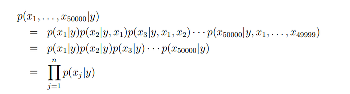
In order to reduce the parameter, we will assume that the xi ’s are conditionally independent given y. This assumption is called the Naive Bayes (NB) assumption, and the resulting algorithm is called the Naive Bayes classifier.
Conditional Independence:
If y = 1 means spam email; “buy” is word 2087 and “price” is word 39831; then we are assuming that y = 1 (spam), then knowledge of X(2087 )(knowledge of whether “buy” appears in the message) will have no effect on your beliefs about the value of X(39831) .
It can be written as:
P(X(2087)|y) = P(X(2087)|y, X(39831)). This means that we are saying X(2087) is independent of X(39831) only in presence of y. This doesn’t mean that p(X(2087)) = p(X(2087)|X(39831))
The first equality simply follows from the usual properties of probabilities. What are the parameters of our model?
φ(j|y=1 )= P(x(j) = 1|y = 1). How come P(z) is parameter? Well it is in terms of Bernoulli distribution p is the parameter. Just like mean and sigma being parameter of Gaussian distribution, p is also a parameter.
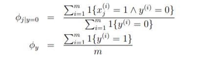
φ(j|y=0 ) = P(x(j) = 1|y = 0)
φ(y) = P(y = 1)
What is the maximum likelihood of them?
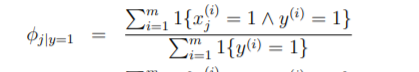
You know what this means? The maximum likelihood of first parameter if our is nothing but all the values where both x and y are 1 divide by total number of y that had 1.
This is what happens in our training phase. Now in testing phase, we go for same discriminative formula of P(y=1|X).
P(y=1|X) = p(x|y = 1)p(y = 1)/ p(x) which can also be written as:
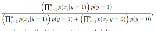
You know what this is, don’t you? Seems so familiar to Bayes theorem? yes it is. I am not delving deeper here.
Laplace Smoothing:
You know you rectify your probability formula for unseen data it is called Laplace Smoothing. Suppose your dictionary doesn’t contain the world ‘Wayne’ but it somehow appeared in your email. Now, the product of probability of text while calculating the P for the email would be 0 because one of its value is 0. So we have to address that thing. Stating the problem more broadly, it is statistically a bad idea to estimate the probability of some event to be zero just because you haven’t seen it before in your finite training set.
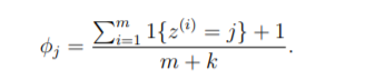
We added 1 in the numerator and k in the denominator. k can be the length of your email texts.