Perceptual Loss — Well it sounds interesting after Neural Style Transfer
Beforehand, we used to find the per pixel loss between predicted image and actual image. This kind of gave us blurry image as result. Therefore we went for style loss which helped us to find the difference between style representation of intermediate layer of both actual and our made up image.
Perceptual loss mixes both these ideas together and make it more reliable for image translations. The per-pixel losses used by these methods do not capture perceptual differences between output and ground-truth images. It’s because the image might look similar in perspective, but they might have different per-pixels values. You see, that is why we cannot depend on per-pixel value.
Recent work has shown that high-quality images can be generated using perceptual loss functions based not on differences between pixels but instead on differences between high-level image feature representations extracted from pretrained CNN. Perceptual losses measure image similarities more robustly than per-pixel losses. The paper is based on doing two tasks.
- Style Transfer
- Super Resolution
Style Transfer which I have previously explained is computationally expensive since each optimization process requires forward and backward pass through pre-trained network. Remember in style transfer how we made our image variable and let network learn it? In Perceptual loss, a feed-forward network is trained.

Actual method:

The figure looks complex. We will break it down. It consists of 2 networks. First network is fW network which is more like encoder-decoder network. The output of that network is y^. Another network is Φ which is pre-trained model from imagenet. We use it for 2 kinds of loss that we will be using. More of this later.
Note: Usage of y^ or ^y is same. Do not confuse yourself.
The image transformation network is a deep residual CNN. It transforms input images x into output images toˆy via the mapping y = f(x).
Each loss function computes a scalar value (y^, yi) measuring the difference between the output image y^ and a target image yi. Remember this. y^ is the output from your residual network, whilst yi is the actual output.
So, our transformation network is f(x). The weights learned by that transformation network will help us to get both super resolution as well as style transfer that we have promised.
Convolutional neural networks pretrained(like imagenet) for image classification have already learned to encode the perceptual and semantic information we would like to measure in our loss functions. So our loss functions depend on the network , the pretrained network.
We got two types of losses:
a) Feature Loss
b) Style Reconstruction Loss
For each input x, we have style target y(s) (remember the style image) and content target y(c). Also remember, that for style transfer, our y(c) and x are same!! (Remember how we used input whose content was transferred to itself and style whose style was transferred to that input in style transfer.)
For super resolution, we use y(c) as high resolution version of input image x. y(s) is not used in super resolution as it is not something we actually care about here.
Image Transformation Network (f(x))
In our Image Transformation Network we use strided convolutions rather than MaxPooling to downsample the image. The architecture is as follows:
All nonresidual convolutional layers are followed by batch normalization and ReLU nonlinearities with the exception of the output layer, which instead uses a scaled tanh to ensure that the output has pixels in the range [0, 255].
The first and last layers use 9×9 kernels; all other convolutional layers use 3×3 kernels.
Inputs:
256*256*3 image => For Style transfer
3*288/f*228/f => For High Resolution where f is upsampling factor
Output:
256*256*3 => For Style Transfer
3×288×288 => For High Resolution
Downsampling and Upsampling:
For super-resolution with an upsampling factor of f, we use several residual blocks followed by logf (base 2) convolutional layers with stride of 0.5.
Fractionally-strided convolution allows the upsampling function to be learned jointly with the rest of the network.
For style transfer our networks use two stride-2 convolutions to downsample the input followed by several residual blocks and then two convolutional layers with stride 1/2 to upsample. It says we use 0.5 stride, but I am not sure whether that is possible.
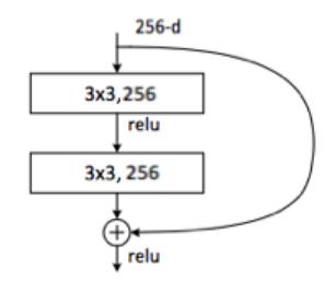
Residual Connection: Residual connections make the identity function easier to learn; this is an appealing property for image transformation networks, since in most cases the output image should share structure with the input image. The body of our network thus consists of several residual blocks.
A residual block is simply when the activation of a layer is fast-forwarded to a deeper layer in the neural network. The network formed from it is called ResNet.


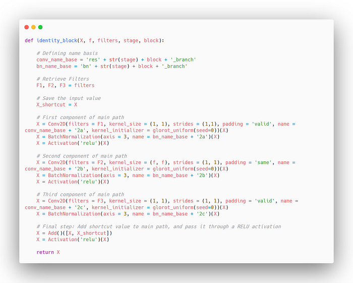
Check the formula here, we saved the X in X_shortcut, and later after forming many actions on that X, we add the new X and X_shortcut. Simple right?
The X and X_shortcut have same shape, else it won’t add up. If it doesn’t add up, then we change X_shortcut molding it to a shape of X (called CONV layer by ResNet) and then add X and X_shortcut.
Perceptual Loss Function: Now this is the most interesting part. We define two perceptual loss functions that measure high-level perceptual and semantic differences between images. As we already know that the loss functions are derived from that of pretrained VGG network which we did in Style Transfer.
Feature Reconstruction Loss:
Rather than telling our transformed network output(y=f(x)) to match up exactly to y(our output image) pixel wise, we encourage them to have similar feature representation, rather than pixels.
Let φj (x) be the activation of the jth layer of the network φ when processing the image x. We know φj (x) is activation map of shape C*H*W. Everything clear upto here right?
The feature reconstruction loss is the euclidean distance between the feature representation of output from transformed network(φj (f(x))); where f(x) is y^. You know y^ is the output from our transformed network; and φj (y); where y is the actual image.

Using a feature reconstruction loss for training our image transformation networks encourages the output image ˆy to be perceptually similar to the target image y, but does not force them to match exactly. I have explained this for about million times. I hope you get this.
In simpler words, Feature Reconstruction loss is similar to style reconstruction loss without the Gram Matrix.
Style Loss:
Not going detail on this, you know about it, you don’t? Check other medium article.
Some other loss functions:
Pixel Loss:
Euclidean distance between output image and predicted image(y^).

This can only be used when when we have a ground-truth target y that the network is expected to match. As far as I know, this won’t be needed in Style Transfer.
Total Variation Regularization:
Here, total variational regularizer is used. l(ˆy).
The total variation is the sum of the absolute differences for neighboring pixel-values in the input images. This measures how much noise is in the images.
This can be used as a loss-function during optimization so as to suppress noise in images. If you have a batch of images, then you should calculate the scalar loss-value as the sum: loss = tf.reduce_sum(tf.image.total_variation(images))
The principle is based on the following theory that: ‘If signal has more noise, it has more variation’. So try to reduce it, means try to reduce the noise.
Style Transfer:
Our first experiment is Style Transfer.
The total loss function including all above losses are as follows:

For Style Transfer, we know that yc = x and y = f(x).
Training Details:
Batch size of 4, for 40k iterations for 80k images for 2 epochs!
Adam Optimizer => Learning rate =1/(10³)
No Weight Decay and Dropout!
For all style transfer, feature reconstruction loss at layer relu3_3 and style reconstruction loss at layers relu1_2, relu2_2, relu3_3, and relu4_3 of the VGG-16 loss network φ. It uses CuDNN for f(W).
The total variation regularization with a strength of between 1 × 010^−6 and 1×10^-4.
I am not doing Super Resolution, so this is what I would do!
I didn’t did this on my laptop, why? Because its boring and doesn’t look worthy of 6–7 hours of my laptop making stupid noise. I will go for STYLE GAN.